本-夏皮罗和龙虾教授的一段访谈

9月1日,本-夏皮罗在自己的博客节目《本-夏皮罗秀》上,采访了著名的“龙虾教授”:乔丹-彼得森。

这期的主题是“如何在自我牺牲中发现美”

在2024年9月1日的《The Ben Shapiro Show》中,Jordan Peterson与Ben Shapiro进行了深入的对话,探讨了自我牺牲之美。Peterson是一位世界知名的临床心理学家、多伦多大学的名誉教授,以及在线教育家,以其关于宗教信仰、叙事神话和人格分析的有影响力的讲座而闻名。在他们的对话中,Peterson分享了他在最新系列《Foundations of the West》中的一些幕后轶事,这个系列中他访问了耶路撒冷、雅典和罗马,以揭示西方文明的古老根源。Peterson还讨论了他的个人宗教旅程,以及他对圣经中风险和牺牲主题的观察。

Peterson在对话中提到了亚伯拉罕和以撒的故事,将其作为牺牲主题的一个例子。他解释说,圣经的叙述挑战了儿童献祭的概念,而是将其呈现为父母必须为孩子做出的牺牲的隐喻。愿意让孩子面对世界,尽管存在固有的危险,是一种自我牺牲,最终导致成长和成熟。这一理念与为了社区和后代而必须做出牺牲的更广泛主题相呼应。

此外,Peterson还讨论了社区和责任的角色,他认为社区本质上是建立在牺牲之上的。他主张,人类经历以关系为特点,这些关系要求个人为了更大的利益做出牺牲。这一概念深深植根于圣经文本中,这些文本始终强调无私和愿意为了秩序而面对混乱的重要性。

Peterson还谈到了这种理解对当代社会的含义。他对日益增长的个人主义趋势和对社区责任的忽视表示担忧。他认为,一个将个人利益置于集体福祉之上的社会,最终会破坏自己的稳定性和道德结构。他建议,圣经的叙述为牺牲的重要性和人类生活的相互联系提供了永恒的智慧。

最后,对话以讨论Peterson在加拿大面临的医疗执照挑战作为高潮,他被政府要求接受社交媒体培训。他表达了对抗的决心,将其视为“反对侵犯言论自由和专业完整性”的道德义务。

这些讨论提供了对自我牺牲、社区责任和个人成长的深刻见解,展示了Peterson对这些主题的深入思考。

大模型vs性象征

我特别感兴趣的一点是:Peterson谈到了大模型对于真实世界的理解(从文本上对世界知识进行压缩),和精神分析中的联想方法(如性象征是更深层次真理的替代品),这两者在某种程度上是相同的(认知领域)。

Peterson说:

“通过阅读弗洛伊德,荣格,埃里克·诺伊曼...如果学术界,如果西方高等教育机构能够采纳诺伊曼...荣格的文学解释方法,我们现在就不会处于文化战争之中了。
他们是对的。我认为我们最终会通过大型语言模型揭示这一点,这已经引起了我的注意,精神分析师通过他们的联想工作,自由联想在梦境解释和叙事解释所做的,与大型语言模型在概念之间统计规律的映射中所做的,从认知领域来看是相同的。
所以最好的思考方式,弗洛伊德认为一个象征,如性象征,是更深层次真理的替代品,这是压抑的结果,对吧?所以压抑的内容会以象征的形式出现。这在很多方面几乎是真的,弗洛伊德所说的许多事情几乎是真的。”

上面这段话很有意思,我不由得猜测,这位龙虾教授难不成被吊销了医疗执照后,打算进军llm行业了?

对于Peterson的看法,我是赞同的。今年8月和同事爬昆明西山,顺便参观了山脚下的美术馆,当时美术馆在展出油画和书法,我靠近观看这张“阳光下的草地”,除了斑驳的颜料色块,是不可能“看到”什么草地、阳光、青山、绿水的。这和我们把人脸图像解析为一串向量数字,没有本质不同,但是当你逐渐拉远距离,会发现灿烂的阳光慢慢浮现,仿佛那时那刻画家眼前的景色重现。

油画就是旧时代的大模型。

*播客地址在此:
From The Ben Shapiro Show: How To Find Beauty In Self-Sacrifice | Jordan Peterson, Sep 1, 2024

力学概论


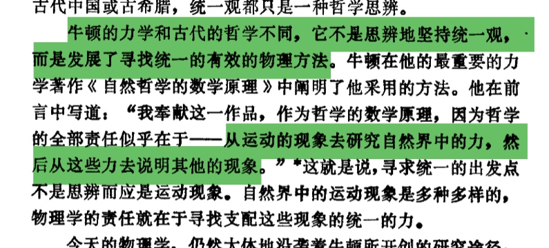
1986年出版的《力学概论》提出,寻求统一的出发点不是思辨而应是运动现象。

我想,之所以方老师这么说,他肯定认为坐而论道是空洞无用的,只有“躬身格物”才是认识世界的唯一正确的道路。

随着llm的出现,我潜意识里,觉得llm也许真是认识这个世界的钥匙,llm是语言的统计学抽象,而语言恰恰是我们认识世界的所有工具的一个表述,当然数学,通过对这个表述的抽象,甚至可以说,是对抽象的进一步抽象,我们可以在更高维度来分析世界面对的真实问题,也许在更高维度里发现的解决方案,也能反过来映射到真实世界中的问题中去。

前几周在昆明西山,参观美术馆里

neo4j的cto描绘知识图谱的光明前景–一篇GraphRAG的宣言

Neo4J的cto,在火热朝天的大模型背景下,是如何来描绘知识图谱价值的呢?

为什么要使用知识图谱

因为不管fine tune还是rag,都不能提供具备一定置信度的正确答案(Vector-based RAG – in the same way as fine-tuning – increases the probability of a correct answer for many kinds of questions. However neither technique provides the certainty of a correct answer.)

把真正的知识(things not strings)与统计的文本技术结合,就能突破天花板。(bring knowledge about things into the mix of statistically-based text techniques)。

使用知识图谱的好处

  1. There’s a robust body of research proving that it gives you better answers to most if not ALL questions you might ask an LLM using normal vector-only RAG.
  2. That alone will be a huge driver of GraphRAG adoption. In addition to that, you get easier development thanks to data being visible when building your app.
  3. A third major advantage is that graphs can be readily understood and reasoned upon by humans as well as machines.

原文链接
https://neo4j.com/blog/graphrag-manifesto/

我的便携火锅,出差有了诗意

2024-07-29 20:52:42 PM

下午刚刚到昆明,带着我的便携式火锅。

早晨特地电话委托前台,帮我预留了面对十字路口的房间,此房间拥有转角落地窗,早晨8点左右,会有强烈的阳光射进来,适合晒背,恰好这次是4楼,更不用担心被路人窥视了。

安顿好行李,沿着十字路口,向云南师范大学的方向,是一个临时的农贸市场,确切的说,是一批违规摆摊的小商小贩,线性排开,大概50米不到的规模,售卖各种水果、玉米、炒货、米糕和各种小菜。

傍晚7点多,刚刚下过小雨,类似我这样买菜的人已然不多,上了年纪的阿姨们,着急把手里的尾货出清,只要我稍作停留,她们就会竭力的推销,3块、3块,当我把目光转向旁边的摊位,马上急促的说到,2块,2块全部拿去。我摇摇头,感觉很抱歉,因为根本不认得这标价2块的菜是什么,看起来是茼蒿吗?用我的小火锅烹饪,会好吃吗,而且这个分量真是不小啊。

旁边摊位,摆着一摞摞小白菜,看起来整整齐齐,干干净净,还未等我开口,阿姨说到,2块,2块,我看看份量,即使非常挥霍,也可以吃2顿,点点头说好,阿姨麻利的用一个小塑料袋装了4颗小白菜,递给我。

返回途中,找了一个超市,用9元购得3包麻辣方便面,可惜火锅调料都有点贵,且量大,会浪费。

这次的经验教训:方便面调料还是太清淡了,第一颗白菜涮好,汤底就寡淡无味了,即使用来泡方便面,也难以称作美味,这两天还是得研究下调味料。

快9点,窗外雨潺潺,隐约的雨声,让此时此刻的生活,有一点点诗意。

华为Ascend NPU适配

Ascend Extension for PyTorch插件

简介

本项目开发了名为torch_npuAscend Extension for PyTorch插件,使昇腾NPU可以适配PyTorch框架,为使用PyTorch框架的开发者提供昇腾AI处理器的超强算力。

昇腾为基于华为昇腾处理器和软件的行业应用及服务提供全栈AI计算基础设施。您可以通过访问昇腾社区,了解关于昇腾的更多信息。

安装

使用二进制文件进行安装

我们为用户提供可以快速安装torch_npu的whl安装包。在安装torch_npu之前,您需要先安装CANN软件。昇腾辅助软件中有更多关于CANN的版本信息。请参考CANN安装指南获取CANN安装包。

  1. 安装PyTorch

通过 pip 安装 PyTorch。

aarch64:

pip3 install torch==2.1.0

x86:

pip3 install torch==2.1.0+cpu  --index-url https://download.pytorch.org/whl/cpu

若使用pip命令安装失败,请使用下载链接或进入PyTorch官方网站进行查询下载对应版本。

架构 Python版本 下载链接
x86 Python3.8 下载链接
x86 Python3.9 下载链接
x86 Python3.10 下载链接
aarch64 Python3.8 下载链接
aarch64 Python3.9 下载链接
aarch64 Python3.10 下载链接
  1. 安装torch_npu依赖

运行以下命令安装依赖。

pip3 install pyyaml
pip3 install setuptools
  1. 安装torch_npu
pip3 install torch-npu==2.1.0.post3

如需要保存安装日志,可在pip3 install命令后面加上参数 --log <PATH>,并对您指定的目录<PATH>做好权限管控。

使用源代码进行安装

某些特殊场景下,用户可能需要自行编译torch_npu。可以根据昇腾辅助软件表PyTorch与Python版本配套表选择合适的分支。推荐使用Docker镜像编译torch_npu,可以通过以下步骤获取(建议只挂载工作路径,并避开系统路径,以降低安全风险), 生成的.whl文件路径为./dist/:

  1. 克隆torch_npu代码仓

    git clone https://gitee.com/ascend/pytorch.git -b v2.1.0-6.0.rc1 --depth 1
    
  2. 构建镜像

    cd pytorch/ci/docker/{arch} # {arch} for X86 or ARM
    docker build -t manylinux-builder:v1 .
    
  3. 进入Docker容器

    docker run -it -v /{code_path}/pytorch:/home/pytorch manylinux-builder:v1 bash
    # {code_path} is the torch_npu source code path
    
  4. 编译torch_npu

    Python 3.8 为例。

    cd /home/pytorch
    bash ci/build.sh --python=3.8
    

卸载

Pytorch框架训练环境的卸载可以参考昇腾官方文档

torch_npu的卸载只需执行命令:

pip3 uninstall torch_npu

如需要保存卸载日志,可在pip3 uninstall命令后面加上参数 --log <PATH>,并对您指定的目录<PATH>做好权限管控。

入门

前提

运行以下命令初始化CANN环境变量。

# Default path, change it if needed.
source /usr/local/Ascend/ascend-toolkit/set_env.sh

快速验证

可以通过以下样例快速体验昇腾NPU

import torch
import torch_npu

x = torch.randn(2, 2).npu()
y = torch.randn(2, 2).npu()
z = x.mm(y)

print(z)

PyTorch与Python版本配套表

PyTorch版本 Python版本
PyTorch1.11.0 Python3.7.x(>=3.7.5), Python3.8.x, Python3.9.x, Python3.10.x
PyTorch2.1.0 Python3.8.x, Python3.9.x, Python3.10.x
PyTorch2.2.0 Python3.8.x, Python3.9.x, Python3.10.x

昇腾辅助软件

PyTorch Extension版本号采用{PyTorch版本}-{昇腾版本}命名规则,前者为PyTorch Extension匹配的PyTorch版本,后者用于匹配CANN版本,详细匹配如下:

CANN版本 支持的PyTorch版本 支持的Extension版本 Gitee分支 AscendHub镜像版本/名称(链接)
CANN 8.0.RC1 2.2.0 2.2.0 v2.2.0-6.0.rc1
2.1.0 2.1.0.post3 v2.1.0-6.0.rc1
1.11.0 1.11.0.post11 v1.11.0-6.0.rc1
CANN 7.0.0 2.1.0 2.1.0 v2.1.0-5.0.0
2.0.1 2.0.1.post1 v2.0.1-5.0.0
1.11.0 1.11.0.post8 v1.11.0-5.0.0
CANN 7.0.RC1 2.1.0 2.1.0.rc1 v2.1.0-5.0.rc3
2.0.1 2.0.1 v2.0.1-5.0.rc3
1.11.0 1.11.0.post4 v1.11.0-5.0.rc3
CANN 6.3.RC3.1 1.11.0 1.11.0.post3 v1.11.0-5.0.rc2.2
CANN 6.3.RC3 1.11.0 1.11.0.post2 v1.11.0-5.0.rc2.1
CANN 6.3.RC2 2.0.1 2.0.1.rc1 v2.0.1-5.0.rc2
1.11.0 1.11.0.post1 v1.11.0-5.0.rc2 23.0.RC1-1.11.0
1.8.1 1.8.1.post2 v1.8.1-5.0.rc2 23.0.RC1-1.8.1
CANN 6.3.RC1 1.11.0 1.11.0 v1.11.0-5.0.rc1
1.8.1 1.8.1.post1 v1.8.1-5.0.rc1
CANN 6.0.1 1.5.0 1.5.0.post8 v1.5.0-3.0.0 22.0.0
1.8.1 1.8.1 v1.8.1-3.0.0 22.0.0-1.8.1
1.11.0 1.11.0.rc2(beta) v1.11.0-3.0.0
CANN 6.0.RC1 1.5.0 1.5.0.post7 v1.5.0-3.0.rc3 22.0.RC3
1.8.1 1.8.1.rc3 v1.8.1-3.0.rc3 22.0.RC3-1.8.1
1.11.0 1.11.0.rc1(beta) v1.11.0-3.0.rc3
CANN 5.1.RC2 1.5.0 1.5.0.post6 v1.5.0-3.0.rc2 22.0.RC2
1.8.1 1.8.1.rc2 v1.8.1-3.0.rc2 22.0.RC2-1.8.1
CANN 5.1.RC1 1.5.0 1.5.0.post5 v1.5.0-3.0.rc1 22.0.RC1
1.8.1 1.8.1.rc1 v1.8.1-3.0.rc1
CANN 5.0.4 1.5.0 1.5.0.post4 2.0.4.tr5 21.0.4
CANN 5.0.3 1.8.1 1.5.0.post3 2.0.3.tr5 21.0.3
CANN 5.0.2 1.5.0 1.5.0.post2 2.0.2.tr5 21.0.2

建议与交流

欢迎大家为社区做贡献。如果有任何疑问或建议,请提交gitee Issues,我们会尽快回复。感谢您的支持。

分支维护策略

AscendPyTorch版本分支的维护阶段如下:

状态 时间 说明
计划 1—3 个月 计划特性
开发 3 个月 开发特性
维护 6-12 个月 合入所有已解决的问题并发布版本,针对不同的PyTorch版本采取不同的维护策略,常规版本和长期支持版本维护周期分别为6个月和12个月
无维护 0—3 个月 合入所有已解决的问题,无专职维护人员,无版本发布
生命周期终止(EOL) N/A 分支不再接受任何修改

PyTorch版本维护策略

PyTorch版本 维护策略 当前状态 发布时间 后续状态 EOL日期
2.2.0 常规版本 维护 2024/04/01 预计2024/10/15起无维护
2.1.0 长期支持 维护 2023/10/15 预计2024/10/15起无维护
2.0.1 常规版本 EOL 2023/7/19 2024/3/14
1.11.0 长期支持 维护 2023/4/19 预计2024/4/19起无维护
1.8.1 长期支持 EOL 2022/4/10 2023/4/10
1.5.0 长期支持 EOL 2021/7/29 2022/7/29

安全声明

Ascend Extension for PyTorch插件 安全声明

参考文档

有关安装指南、模型迁移和训练/推理教程和API列表等更多详细信息,请参考昇腾社区Ascend Extension for PyTorch

文档名称 文档链接
安装指南 参考链接
网络模型迁移和训练 参考链接
算子适配 参考链接
API清单(PyTorch原生接口与自定义接口) 参考链接

许可证

Ascend Extension for PyTorch插件使用BSD许可证。详见LICENSE文件。

在colab里跑书生大模型

1.8B(fp16情况下,3.35G)跑下来没有问题。

下图是20B模型(fp16情况下,37G),把环境搞宕机了,硬盘只有78G,我尝试挂载一块google drive上去是否可行。

计算逻辑

要计算使用 fp16(半精度浮点数)时 InternLM 20B 模型的大小,我们可以按照以下步骤进行:

参数数量:

InternLM 20B 模型包含 20B(20,000,000,000)个参数。
每个参数的大小:

在 fp16 模式下,每个浮点数占用 2 个字节(16 位)。
计算模型大小:

模型大小(字节) = 参数数量 × 每个参数的大小(字节)
模型大小(字节) = 20,000,000,000 × 2
模型大小(字节) = 40,000,000,000 字节
转换为常见单位:

1 GB = 1,073,741,824 字节
模型大小(GB) = 模型大小(字节) / 1,073,741,824
模型大小(GB) ≈ 40,000,000,000 / 1,073,741,824
模型大小(GB) ≈ 37.25 GB
结果
在 fp16 模式下,InternLM 20B 模型的大小约为 37.25 GB。

这个计算基于每个参数占用 2 个字节的假设,并且忽略了模型中的额外开销(例如优化器状态和其他元数据),所以实际的内存占用可能略高。

文本向量化和停止词

我在准备文本向量化过程中,发现有几个单词没有作为特征被提取出来,比如说“I”

ChatGPT回答,这应该是向量工具有一套默认的英文停止词,例如i,the等等,如果要确保去除stop words的影响,可以在方法中添加一个参数。
The word "I" is missing from the feature names because CountVectorizer by default removes English stop words, which are common words like "I", "the", "is", etc., that are often filtered out because they do not contain significant meaning in the context of text analysis.

from sklearn.feature_extraction.text import CountVectorizer

# Sample text data
documents = [
    "I love programming in Python",
    "Python is a great language",
    "I love coding"
]

# Create an instance of CountVectorizer without stop words removal
# 注意!!!在这里的参数意味不要使用停止词!!!
vect = CountVectorizer(stop_words=None)

# Fit and transform the data
X = vect.fit_transform(documents)

# Convert to dense array
X_dense = X.toarray()

# Get feature names (tokens)
feature_names = vect.get_feature_names_out()

# Print feature names and the dense array for verification
print("Feature names:", feature_names)
print("Dense array:\n", X_dense)

# Sum the counts of each token across all documents
token_counts = X_dense.sum(axis=0)

# Create a dictionary of tokens and their counts
token_count_dict = dict(zip(feature_names, token_counts))

# Print the token counts
for token, count in token_count_dict.items():
    print(f"{token}: {count}")

下面是新的输出结果

Feature names: ['coding' 'great' 'i' 'in' 'is' 'language' 'love' 'programming' 'python']
Dense array:
 [[0 0 1 1 0 0 1 1 1]
  [0 1 0 1 1 1 0 0 1]
  [1 0 1 0 0 0 1 0 0]]
coding: 1
great: 1
i: 2
in: 1
is: 1
language: 1
love: 2
programming: 1
python: 2

文本向量化和词频,以及稀疏矩阵和稠密矩阵

文本向量化和词频统计示例

下面的代码把一个文档,转化成稀疏矩阵,然后为了更通俗易懂的处理(同时部分算法也不支持稀疏矩阵),再把它转化为稠密矩阵

from sklearn.feature_extraction.text import CountVectorizer

# Sample text data
documents = [
    "I love programming in Python",
    "Python is a great language",
    "I love coding"
]

# Create an instance of CountVectorizer
vect = CountVectorizer()

# Fit and transform the data
X = vect.fit_transform(documents)

# Convert to dense array
X_dense = X.toarray()

# Get feature names (tokens)
feature_names = vect.get_feature_names_out()

# Print feature names and the dense array for verification
print("Feature names:", feature_names)
print("Dense array:\n", X_dense)

# Sum the counts of each token across all documents
token_counts = X_dense.sum(axis=0)

# Create a dictionary of tokens and their counts
token_count_dict = dict(zip(feature_names, token_counts))

# Print the token counts
for token, count in token_count_dict.items():
    print(f"{token}: {count}")

输出的结果如下

This example will print the feature names, the dense array, and the token counts:

Feature names: ['coding' 'great' 'in' 'is' 'language' 'love' 'programming' 'python']
Dense array:
 [[0 0 0 0 0 1 1 1]
  [0 1 1 1 1 0 0 1]
  [1 0 0 0 0 1 0 0]]
coding: 1
great: 1
in: 1
is: 1
language: 1
love: 2
programming: 1
python: 2

Explanation of the Output

Feature Names:

The feature names are printed in the same order as they appear in the dense array’s columns: [‘coding’ ‘great’ ‘in’ ‘is’ ‘language’ ‘love’ ‘programming’ ‘python’].
Dense Array:

The dense array shows the token counts for each document, with each column corresponding to the respective feature name.
For example, the first column corresponds to ‘coding’, the second column to ‘great’, and so on.
Token Counts:

The token counts dictionary shows the total count of each token across all documents, matching the counts in the dense array.
Verification
To verify the correspondence, look at the dense array and the feature names:

The first column in X_dense corresponds to ‘coding’. In the dense array, the first column has counts [0, 0, 1], meaning ‘coding’ appears once in the third document.
The second column corresponds to ‘great’. The counts are [0, 1, 0], meaning ‘great’ appears once in the second document.
This pattern continues for all feature names and their corresponding columns.
Conclusion
The sequence of the feature names is the same as the columns of the dense array. Each column in the dense array represents the count of a specific token, and the order of these tokens is given by feature_names.

Sparse Matrix vs. Dense Array

When using CountVectorizer to transform text data into a matrix of token counts, the result is a sparse matrix by default. Let’s explore the differences between sparse matrices and dense arrays, and why one might be preferred over the other in certain contexts.

Sparse Matrix

A sparse matrix is a matrix in which most of the elements are zero. Instead of storing every element, sparse matrices store only the non-zero elements and their positions. This can lead to significant memory savings when dealing with large datasets where the number of zeros vastly outnumbers the number of non-zero elements.

Advantages:
Memory Efficiency: Sparse matrices save memory by only storing non-zero elements. This is crucial for large datasets with many features (e.g., in text processing where there are many words but each document only contains a small subset).
Performance: Certain operations can be faster on sparse matrices due to the reduced amount of data.
Disadvantages:
Complexity: Sparse matrices are more complex to manipulate and understand because they don’t store data in a straightforward row-by-row manner.

Dense Array

A dense array, on the other hand, stores all elements explicitly, including the zero elements. This means it takes up more memory but is simpler to understand and manipulate.

Advantages:
Simplicity: Dense arrays are easier to work with because they store data in a straightforward manner, where each element corresponds directly to a position in the matrix.
Compatibility: Some algorithms and libraries work only with dense arrays, not sparse matrices.
Disadvantages:
Memory Usage: Dense arrays can consume a lot of memory if the dataset is large and contains many zero elements.

示例解释

Interpretation
Sparse Matrix:

Efficiently stores data when most elements are zero.
Example representation (only showing non-zero values and their positions):
scss

(0, 4) 1
(0, 7) 1
(0, 8) 1
(0, 5) 1
(0, 6) 1
(1, 4) 1
(1, 2) 1
(1, 1) 1
(1, 3) 1
(2, 5) 1
(2, 0) 1
(2, 6) 1

Dense Array:

Simpler to understand as it stores all elements explicitly.
Example representation:

[[0 0 0 1 1 0 1 1 1]
 [0 0 1 0 1 1 0 0 0]
 [1 0 0 0 0 1 1 0 0]]

Each row corresponds to a document, and each column corresponds to a token. The values represent the count of each token in the respective document.

In summary, sparse matrices are memory-efficient and suitable for large datasets with many zero elements, while dense arrays are straightforward and easier to work with for smaller datasets or when simplicity is desired.

来自Kimi的中文解释

在计算机科学和数学中,稀疏矩阵和稠密矩阵是两种不同类型的矩阵,它们在存储和处理上有所不同,主要取决于矩阵中非零元素的数量。

稠密矩阵(Dense Matrix)

稠密矩阵是指大多数元素都是非零的矩阵。在稠密矩阵中,非零元素的数量接近于矩阵的总元素数量。稠密矩阵通常使用完整的二维数组来表示,每个元素都有一个对应的存储空间。

特点

  • 存储需求较大,因为每个元素都需要存储空间。
  • 矩阵操作(如加法、乘法等)通常需要更多的计算资源。
  • 在数据分析、图像处理等领域中,当数据集中的非零元素较多时,稠密矩阵较为常见。

稀疏矩阵(Sparse Matrix)

稀疏矩阵是指矩阵中大部分元素都是零的矩阵。在稀疏矩阵中,非零元素的数量远小于矩阵的总元素数量。为了节省存储空间和提高计算效率,稀疏矩阵通常不会使用完整的二维数组来存储,而是使用特殊的数据结构来存储非零元素和它们的位置信息。

特点

  • 存储需求较小,因为只有非零元素和它们的位置需要存储。
  • 矩阵操作可以更高效,因为可以忽略大量的零元素。
  • 在许多应用中非常常见,如文本处理(词频矩阵)、社交网络分析、大规模数值模拟等。

稀疏矩阵的存储方式

  • 三元组列表(Triplet List):存储所有非零元素及其行索引和列索引的列表。
  • 压缩存储格式:通常分为两种,行压缩存储(Compressed Sparse Row, CSR)和列压缩存储(Compressed Sparse Column, CSC)。
    • CSR:按行压缩存储,适合行操作。
    • CSC:按列压缩存储,适合列操作。
  • 坐标列表(Coordinate List):类似于三元组列表,但通常不按行或列排序。

在实际应用中,选择使用稀疏矩阵还是稠密矩阵取决于具体问题的需求和数据的特点。稀疏矩阵在处理大规模稀疏数据时具有明显的优势,可以显著减少存储需求和提高计算效率。而稠密矩阵则适用于大多数元素都需要参与计算的情况。

神奇数字“42”

The choice of random_state=42 is somewhat of a cultural reference and an inside joke in the programming and data science community. Here’s the background and explanation:

Why 42?

Cultural Reference:
The number 42 is famously known as "the answer to the ultimate question of life, the universe, and everything" from Douglas Adams’ science fiction series "The Hitchhiker’s Guide to the Galaxy". This reference has made the number 42 a playful, arbitrary choice that many programmers and data scientists use when a random seed is needed.
Consistency:
Since many tutorials and examples use 42, it has become a de facto standard. Using the same random seed can make it easier for others to follow along with examples and verify results.